NumPy Library Tutorial 2026

Installing Numpy

You need to set up a virtual environment in Python. You need to install virtualenv. If you are using pip, run the command below:

pip install virtualenv

If you are using pip3, use pip3 instead of pip.

You need to create a virtual environment in your Python project folder. If you are using pip, run the command below:

python -m venv new_env

If you are using python3, use python3 instead of python. We named the virtual environment "new_env" but you can choose another name.

You can activate the environment:

source new_env/bin/activate

If you are using pip, run the command below:

pip install numpy

If you are using conda, run the command below:

conda install numpy

To check the version of NumPy library:

import numpy as np
print(np.__version__)

NumPy 2.0.0 will be used in the tutorial below. When you install with the command above, the latest version will be installed.

Matplotlib library will be used in the tutorial. You can install seaborn and pandas as well. If you are using pip, run the commands below:

pip install seaborn

pip install pandas

pip install matplotlib

If you are using conda, run the commands below:

conda install seaborn

conda install pandas

conda install -c conda-forge matplotlib

Import the seaborn and other libraries:

import matplotlib.pyplot as plt
import seaborn as sns
import numpy as np

NumPy Arrays, N-dimensional arrays

Creating arrays

Let's create a NumPy array:

arr = np.array([1, 2, 3])

The NumPy array above is one dimensional, you can also create a two-dimensional array:

arr = np.array([[1, 2, 3], [4, 5, 6]])

You can also import a CSV file:

np.genfromtxt('sample.csv', delimiter=',')

You can add more dimensions. You can also check the number of dimensions:

import numpy as np
print(arr.ndim)

You can create an array with the number of dimensions:

arr = np.array([1, 2, 3, 4], ndmin=5)
print(arr)

[[[[[1 2 3 4]]]]]

zeros()

You can create a NumPy array with zeros() function:

print(np.zeros([3, 2], dtype = np.int32))

[[0 0]
[0 0]
[0 0]]

The zeros() function returns a new array of given shape and types, filled with zeros like in the example above.

dtype property shows the data type. dtype can also be used to learn the data type of a variable:

x = np.ones([2, 2], dtype = np.int32)
print(x.dtype)

int32

If you want to change the data type, you can use astype property:

x = np.ones([2, 2], dtype = np.int32)
print("The first data type is ", x.dtype)
x = x.astype("float64")
print("The second data type is ", x.dtype)

The first data type is int32
The second data type is float64

ones()

You can create a NumPy array with np.ones() function:

print(np.ones([2, 2], dtype = np.int32))

[[1 1]
[1 1]]

np.ones() function returns a new array of given shape and type, filled with ones like in the example above.

full()

The np.full() returns a new array of given shape and types, filled with the specified value:

print(np.full([2, 2], 9))

[[9 9]
[9 9]]

Accessing elements

arr = np.array([1, 2, 3, 4])
print(arr[2])

The result is 3.

arr = np.array([[1,2,3,4,5], [6,7,8,9,10]])
print(arr[0, 1])

It represents the second element of the first array. The result is 2.

Please note that a two-dimensional array has two axes: axis 0 represents the column (values in the same column) and axis 1 represents the row (the values in the same row/array).

Slicing

You can slice arrays:

arr = np.array([1,2,3,4,5])
print(arr[1:3])

The result is [2,3]. You can also add a step:

arr = np.array([1,2,3,4,5])
print(arr[1:3:2])

The result is [2]

Logical Operators

You can also use logical operators:

arr = np.array([1, 3, 5, 7, 9, 11])
print(arr[arr>5])

[ 7 9 11]

arr = np.array([1, 3, 5, 7, 9, 11])
print(arr[(arr > 7) | (arr < 5)] )

[ 1 3 9 11]

Changing shape of an array

You can check the shape of an array:

print(arr.shape)

There are different ways to reshape an array. You can use reshape method to change the array. For example, you can change the dimension of an array:

arr = np.array([1, 2, 3, 4, 5, 6, 7, 8, 9])
new_arr = arr.reshape(3,3)
print(new_arr)

[[1 2 3]
[4 5 6]
[7 8 9]]

reshape method changes the dimensions of the first array.

You can also flatten an array:

arr = np.array([[1, 2], [3, 4]])
newarr = arr.reshape(-1)
print(newarr)

[1 2 3 4]

Operations with Numpy Arrays

There are different ways to perform an operation on arrays. For example, you can make an operation for all the elements in an array:

arr = np.array([1,3,5,7])
new_arr = arr + 2
print(new_arr)

[3 5 7 9]

Elements of arrays can also be added to each other:

test_1 = np.array([9, 9, 8, 1, 8])
test_2 = np.array([7, 10, 8, 3, 1])
test_3 = test_1 + test_2
print(test_3)

[16 19 16 4 9]

Universal Functions (ufunc)

A universal function (ufunc) is a function that operates on ndarrays. A ufunc takes a fixed number of specific inputs and produces a fixed number of specific outputs. ufuncs can also take optional arguments: where, dtype, and out (output array where the return value should be copied). There are currently more than 60 universal functions defined in numpy.

Math operations

You can use np.add(), np.subtract(), np.multiply(), np.divide(), np.power(), np.remainder(), np.divmod(), and the np.absolute() functions. You can use the same syntax for all functions. Let's see some of them:

add()

The np.add() function sums the content of two arrays, and returns the results in a new array.

import numpy as np
arr_1 = np.array([9, 9, 8, 1, 8])
arr_2 = np.array([7, 10, 8, 3, 1])
arr_3 = np.add(arr_1, arr_2)
print(arr_3)

[16 19 16 4 9]

power()

The first array elements are raised to powers from the second array elements in the np.power() method.

x = [1, 2, 3, 4]
y = [2, 4, 1, 3]
k = np.power(x,y)
print(k)

[ 1 16 3 64]

You need to calculate [1²   2⁴   3¹   4³] for the result above.

remainder()

The np.remainder() returns the element-wise remainder of the division.

arr_1 = np.array([9, 6, 8, 7, 5])
arr_2 = np.array([7, 3, 2, 3, 4])
arr_3 = np.remainder(arr_1, arr_2)
print(arr_3)

[2 0 0 1 1]

You can get the same result with the mod() function.

divmod()

The np.divmod() returns the element-wise quotient and remainder simultaneously.

arr_1 = np.array([9, 6, 8, 7, 5])
arr_2 = np.array([7, 3, 2, 3, 4])
arr_3 = np.divmod(arr_1, arr_2)
print(arr_3)

(array([1, 2, 4, 2, 1]), array([2, 0, 0, 1, 1]))

absolute()

The np.abs() method calculates the absolute value element-wise.

arr_1 = np.array([-9, -6, -8, -7, -5])
new_arr = np.abs(arr_1)
print(new_arr)

[9 6 8 7 5]

Rounding decimals

You can use truncation, fix, round, floor, and ceil functions for rounding decimals.

trunc()

numpy.trunc() rounds to the nearest integer towards zero.

arr_1 = np.array([1.3, 2.5, 4.6])
new_arr = np.trunc(arr_1)
print(new_arr)

[1. 2. 4.]

You can get the same result with the numpy.fix() function.

floor()

The np.floor() function rounds off decimals to the nearest lower integer.

arr_1 = np.array([-1.3, -2.5, -4.6])
new_arr = np.floor(arr_1)
print(new_arr)

[-2. -3. -5.]

round()

The np.round() evenly rounds to the given number of decimals.

arr_1 = np.array([-1.34685, -2.54232, -4.64242])
new_arr = np.round(arr_1, 2)
print(new_arr)

[-1.35 -2.54 -4.64]

ceil()

The np.ceil() returns the ceiling of the input, element-wise:

arr_1 = np.array([-1.3, -2.5, -4.6])
new_arr = np.ceil(arr_1)
print(new_arr)

[-1. -2. -4.]

Logs

You can use log base 2 or 10 of the given array:

import numpy as np
arr = np.arange(1, 8)
print(np.log2(arr))

*numpy.arange returns evenly spaced values within a given interval.

[0. 1. 1.5849625 2. 2.32192809 2.5849625 2.80735492]

log base 10:

import numpy as np
arr = np.array([10, 100, 1000])
print(np.log10(arr))

[1. 2. 3.]

The natural logarithm is the inverse of the exponential function.

Summation

sum()

The np.sum() calculates the sum of array elements over a given axis:

arr_1 = np.array([3, 2, 4])
new_arr = np.sum(arr_1)
print(new_arr)

The result is 9. Please note that np.sum() and np.add() functions are different.

You can also sum over an axis:

arr_1 = np.array([3, 2, 4])
arr_2 = np.array([3, 2, 4])
new_arr = np.sum([arr_1, arr_2], axis=1)
print(new_arr)

[9 9]

cumsum()

The np.cumsum() returns the cumulative sum of the elements along a given axis.

arr = np.array([2, 4, 6])
new_arr = np.cumsum(arr)
print(new_arr)

[ 2 6 12]

Products

prod()

The np.prod() returns the product of array elements over a given axis.

arr1 = np.array([1, 2, 3, 4])
arr2 = np.array([1, 2, 3, 4])
x = np.prod([arr1, arr2])
print(x)

The result (1 * 2 * 3 * 4 * 1 * 2 * 3 * 4) is 576.

Differences

diff()

The np.diff() method calculates the n-th discrete difference along the given axis.

arr1 = np.array([1, 2, 3, 4])
x = np.diff(arr1)
print(x)

The result is [1 1 1] because 2-1=1, 3-2=1, 4-3=1.

Finding Lowest Common Multiple (LCM) and Greatest Common Denominator (GCD)

Finding Lowest Common Multiple (LCM)

The np.lcm() returns the lowest common multiple of the array:

arr = np.array([4, 5, 20])
x = np.lcm.reduce(arr)
print(x)

The result is 20.

Greatest Common Denominator (GCD)

The numpy.gcd() returns the greatest common divisor of two elements:

arr = np.array([4, 8, 12])
x = np.gcd.reduce(arr)
print(x)

The result is 4.

Set operations

A set in mathematics is a collection of unique elements. You can use unique method to find unique elements from an array:

arr = np.array([4, 8, 12, 4, 6, 8])
x = np.unique(arr)
print(x)

[ 4 6 8 12]

The set arrays can have only one dimension.

Finding union union1d()

numpy.union1d() finds the union of two arrays.

arr = np.array([4, 8, 12])
arr2 = np.array([4,9,15])
x = np.union1d(arr, arr2)
print(x)

[ 4 8 9 12 15]

np.union1d joins the two arrays. As it's a set array, common elements don't repeat.

Finding intersection intersect1d()

np.intersect1d() finds the intersection of two arrays.

arr = np.array([4, 8, 12])
arr2 = np.array([4,9,15])
x = np.intersect1d(arr, arr2)
print(x)

[4]

Finding Difference setdiff1d()

np.setdiff1d() finds the set difference of two arrays. It returns the unique values in the first array that are not in the second array.

arr = np.array([4, 8, 12])
arr2 = np.array([4,9,15])
x = np.setdiff1d(arr, arr2)
print(x)

[ 8 12]

Finding Symmetric Difference setxor1d()

np.setxor1d() finds the set exclusive-or of two arrays.

arr = np.array([4, 8, 12])
arr2 = np.array([4,9,15])
x = np.setxor1d(arr, arr2)
print(x)

[ 8 9 12 15]

setxor1d returns the unique values of two arrays.

Please note that functions always return sorted, unique values.

Create your own ufunc

frompyfunc()

The numpy.frompyfunc helps you create your ufunc. It takes 3 arguments: the name of the function, the number of input array(s) and the number of output array(s).

def subt(x, y):
  return x-y
subt = np.frompyfunc(subt, 2, 1)
print(subt([8, 7, 6], [3, 2, 1]))

[5 5 5]

Statistics with NumPy

You can use NumPy to analyze the data. You can find examples of the numpy mean, numpy median, numpy sort, numpy percentile, and numpy standard deviation methods below. They are used in statistics and machine learning.

mean()

The np.mean() computes the arithmetic mean along the specified axis.

x = np.array([8, 7, 6, 3, 2, 1])
y = np.mean(x)
print(y)

The result is 4.5

median()

The np.median() computes the median along the specified axis.

x = np.array([8, 7, 6, 3, 2, 1])
y = np.median(x)
print(y)

The result is 4.5

While the np.mean shows the average value of the elements in an array, the np.median shows the middle value. median is the data value in the middle of the set (when the array is sorted). If the total number of the array is even, average of the 2 data values in the middle is the median.

sort()

We can use the np.sort() function to sort a Numpy array:

x = np.array([12, 15, 59, 9, 2, 10])
print(np.sort(x))

[ 2 9 10 12 15 59]

percentile

The np.percentile computes the q-th percentile of the data along the specified axis. It returns the q-th percentile(s) of the array elements.

x = np.array([1, 3, 5, 7, 9])
y = np.percentile(x, 25)
print(y)

The result is 3.0

standard deviation

np.std() computes the standard deviation — a measure of the spread or dispersion of a distribution — for the elements in an array along the specified axis.

x = np.array([1, 3, 5, 7, 9])
y = np.std(x)
print(y)

The result is 2.8284271247461903

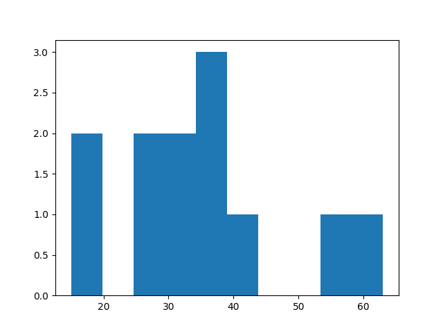
Histogram

You can use a histogram with NumPy. You will need matplotlib:

import numpy as np
from matplotlib import pyplot as plt

number_of_visitors = np.array([15, 25, 30, 54, 43, 35, 63, 37, 18, 28, 30, 35])
plt.hist(number_of_visitors)
plt.show()

Linear Algebra with NumPy (numpy.linalg)

If you're ready to go beyond the basics, our NumPy Linear Algebra Guide dives deep into matrix operations, eigenvalues and eigenvectors, matrix decompositions like SVD, QR, and Cholesky, and practical applications such as least squares and covariance analysis. This tutorial is perfect for anyone looking to strengthen their understanding of linear algebra in Python, optimize matrix computations, and apply these techniques in data science, machine learning, and scientific computing. Explore the full Linear Algebra with Numpy guide to take your NumPy skills to the next level.